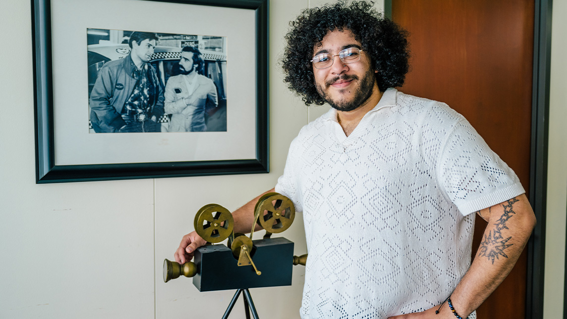
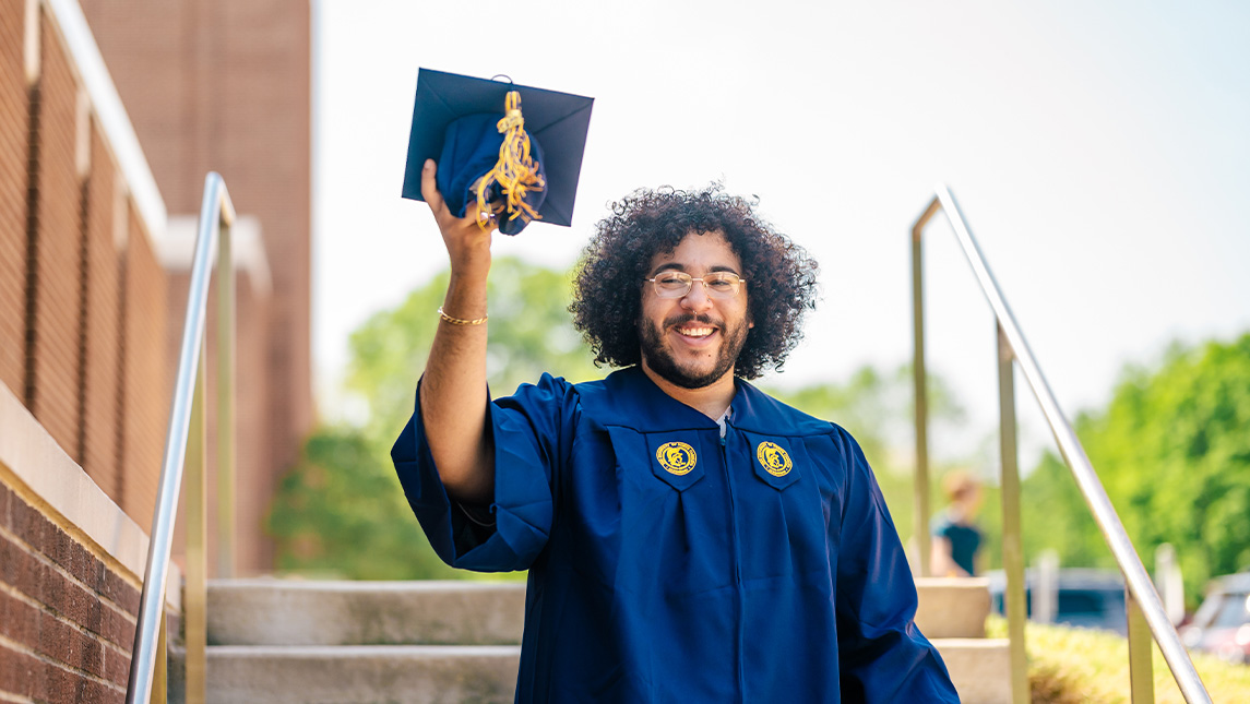
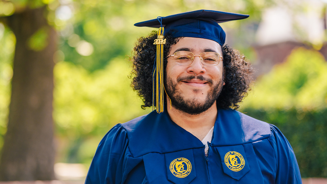
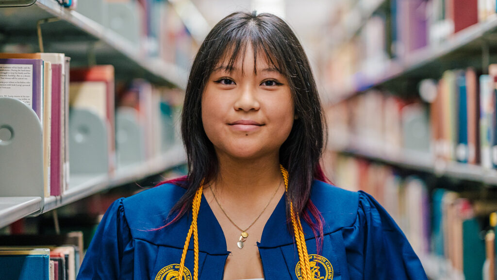
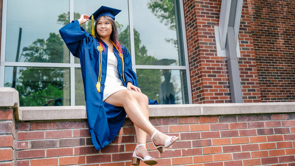
When Tiffany Tan graduates from UNC Greensboro in May 2024, she’ll earn two degrees: a bachelor of arts in studio art and a bachelor of science in psychology, but doctoral studies are already on her horizon.
“I heard it’s unusual for students to get into a PhD program right after earning their bachelor’s degree,” says Tan, who is already accepted into the University of Kansas’s counseling psychology PhD program.
The arduous application process included a personal statement, three letters of recommendation, a CV, and an explanation of leadership experience. Tan applied to eight schools for her doctoral studies, receiving one preliminary interview and two formal interviews for spots in counseling psychology programs – ultimately going with the University of Kansas. Her achievement would not have been possible without her hard work and opportunities presented to her at UNCG.
CERAMICS MIXED WITH PSYCHOLOGY
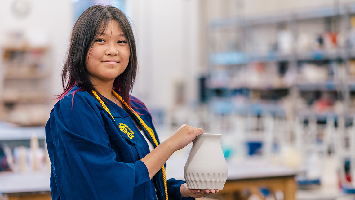
Tan, who is originally from Chapel Hill, North Carolina, has loved art since high school. Her high school art teacher, a UNCG alumna, encouraged a love for ceramics and led Tan to tour UNCG’s Gatewood Studio Center. UNCG was one of only two schools Tan applied to, with some encouragement from her mother as well – another UNCG alumna.
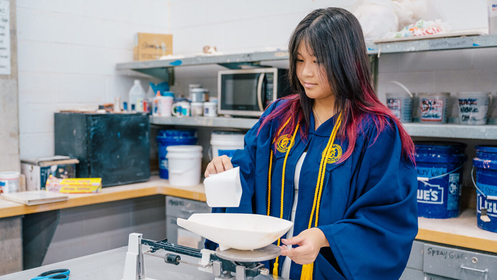
“The Gatewood Studio Arts Center was very impressive and it solidified my decision to come here,” says Tan, who would later become a CVPA student ambassador to help other students see the benefit of the G. “The ceramics classes have been my favorite. You start with hand building, then wheel throwing and then slip casting. There’s something for everyone. There’s also a lot of non-art students taking the classes, so I’ve been able to make connections there as well.”
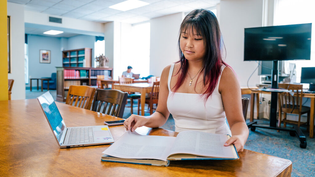
Tan began as a studio arts major with a focus in ceramics, but a general psychology class changed the direction of her education – adding psychology as a major. Tan is in the Lloyd International Honors College and was also the recipient of the Mildred Millner Alvarez Endowed Undergraduate Scholarship in Psychology. Her thesis focuses on minority mental health and academic achievement, specifically how college students of color talk with their parents about race, emotions, and academics.
ON THE RIGHT “CAMINO”
Her work with Dr. Gabriela Livas Stein in the CAMINOS Lab, a clinical psychology research lab at UNCG, sparked her interest in the thesis topic. Stein runs the lab which works to identify individual, familial, and cultural processes that place minoritized youth at risk of maladaptive psychological and education outcomes, focusing on immigrant and Latinx populations.
“We have been so grateful to have Tiffany working with the CAMINOS lab,” says Livas Stein. “She helped shape three different research projects that considered the experiences of racial-ethnic minority families in the US, and she developed a novel honor’s thesis that she presented at an international conference for the Society for Research on Adolescence. However, her contribution to class has been the most impactful as she is curious, insightful, collaborative, and passionate during discussions, and supportive and encouraging of her peers.”
UNCG’s Undergraduate Research, Scholarship, and Creativity (URSCO) funded Tan’s travel to the Society for Research on Adolescence Conference.
“The mentorship in the Caminos Lab is a standout from my time at UNCG,” says Tan. “Being able to have first-hand research experience and also having support from the URSCO has been great.”
A PSYCHOLOGY STANDOUT
Other faculty also helped Tan develop her thesis, specifically the Director of the Psychology Honors Program Dr. Janet Boseovski.
“We worked really closely with her, specifically on how to do a literature review and also talked about diversity and psychology’s history in general so we could have an inclusive process and measures in our study,” says Tan.
“Tiffany is a top student in the disciplinary honors program. She demonstrated strong conceptual knowledge about the field in general and on her project topic on psychological costs associated with resilience in minority youth. She is an excellent academic writer and has strong speaking skills,” says Boseovski.
Tan’s hard work has also caught the attention of University leadership. In November 2023, she was chosen as a student representative at the joint UNC System Board of Governors and UNCG Board of Trustees meeting held at UNCG. The meeting included members of both boards, along with Chancellors from each of the UNC System institutions.
“I had the opportunity to speak with Chancellors from other universities and tell them about my UNCG experience and what my future plans are,” says Tan. “I even heard from one of the Chancellors who said he didn’t know how his school would top UNCG when it was his turn to host the event. It was very cool.”
Not only did she encourage prospective students to choose UNCG, Tan also worked to help fellow students succeed by tutoring in psychology and serving as a psychology peer advisor.
“Tiffany’s generous nature stands out just as much as her academic accomplishments: she was extremely supportive of her classmates and consistently offered constructive and encouraging feedback in class presentations,” says Boseovski. “She is an exemplary ambassador of the department and UNCG on the whole.”
Looking forward, Tan’s spirit of service to others will continue.
“I’m excited for what’s ahead with my PhD program. Lawrence, Kansas, where the University of Kansas is located, has a similar vibe to my hometown. Regardless of how long it takes, I would like to become a tenure-track professor in academia.”
Story by Avery Craine Powell, University Communications
Photography by Sean Norona, University Communications
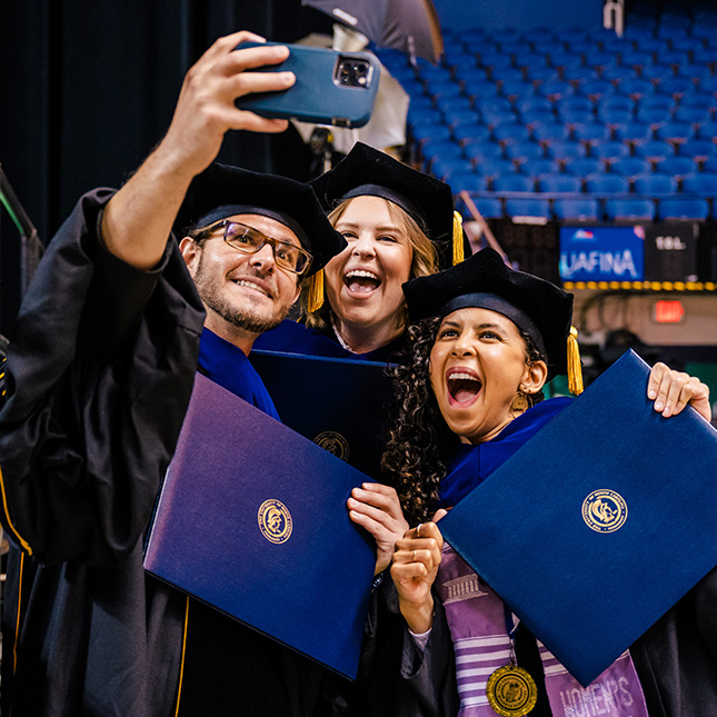
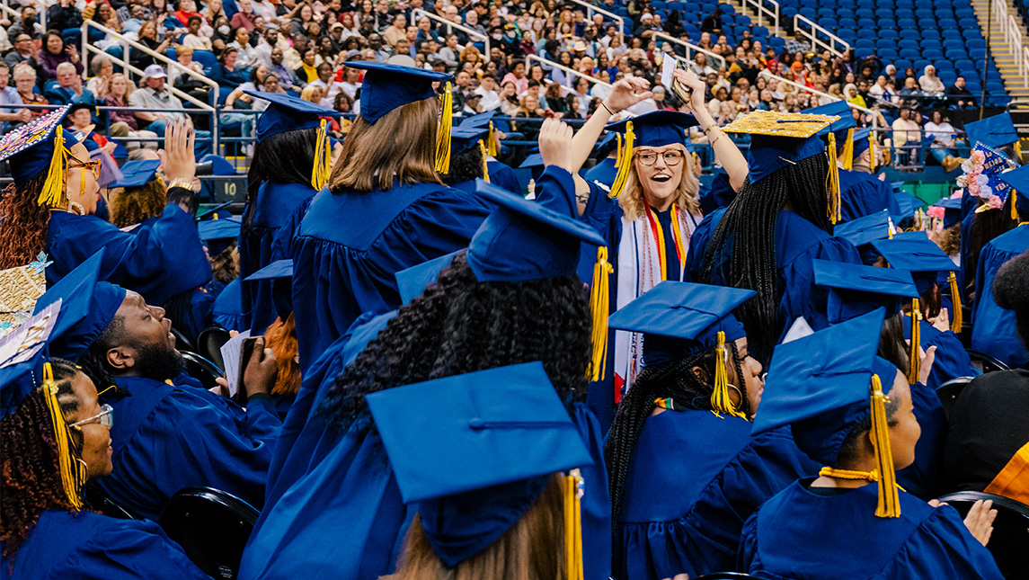
CELEBRATE OUR GRADS!
Graduate Commencement: May 2 at the Greensboro Coliseum
Undergraduate Commencement: May 3 at the Greensboro Coliseum
Graduates and their families are encouraged to share their accomplishments on social media by tagging the University accounts and using the hashtags #UNCGGrad and #UNCGWay. Visit UNCG’s digital swag page for graduation-themed graphics, filters, and templates.
Mention @UNCG in celebratory posts on Instagram and X and @uncgreensboro on TikTok.