Engage with peers and UNC Greensboro’s stellar faculty and staff in a variety of arts, gaming, technology, science, music, or athletics camps hosted at the University.
UNCG offers various camps to promote the academic interests of youth in the community and help them build critical motor and social skills.
Here’s a list of some of the camps provided this summer, and how to register:
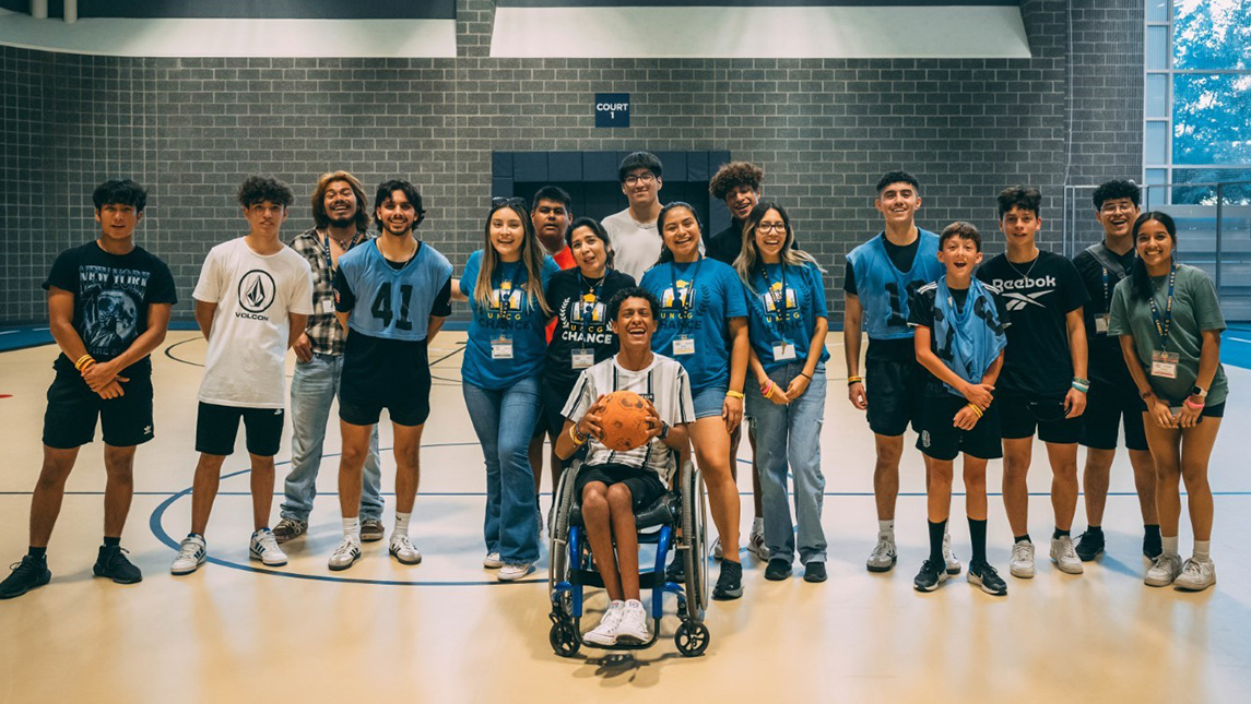
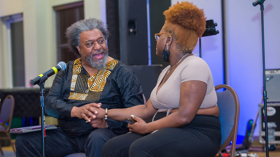
“CHANCE is so much more than just a camp. For once in my life, an educational institution acknowledged me. They acknowledged my community. They recognized our barriers, our struggles, our efforts.”
Grecia Navarro, CHANCE volunteer
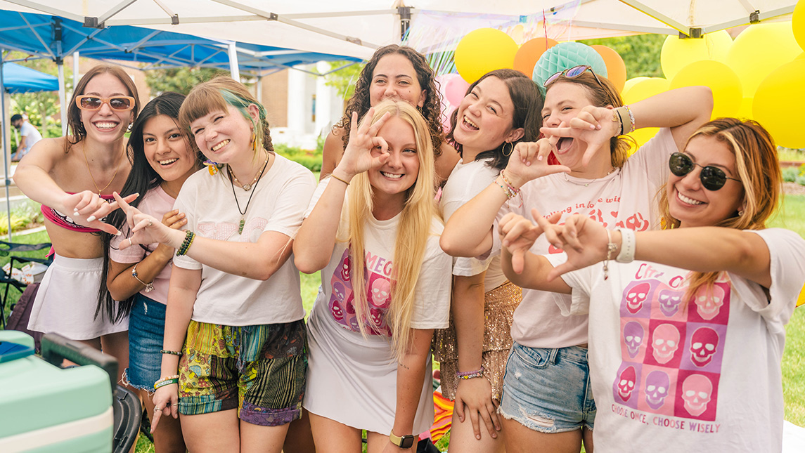
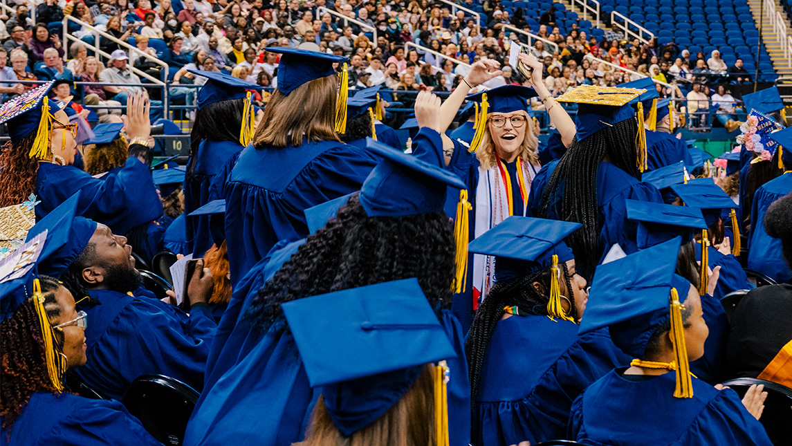
CHANCE camp
CHANCE is a four-day summer program for Latino and Hispanic high school students. CHANCE aims to equip them with the knowledge and skills to advance their education with UNCG as a school of choice. At CHANCE, campers live in a residence hall, eat in the dining hall, and learn more about the resources and opportunities UNCG has to offer. The dates for CHANCE camp are July 17 – 20.
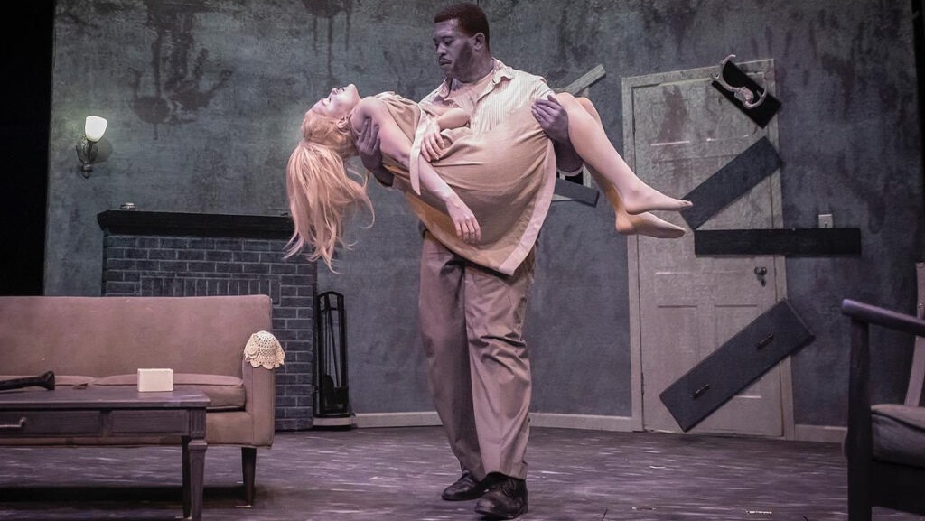
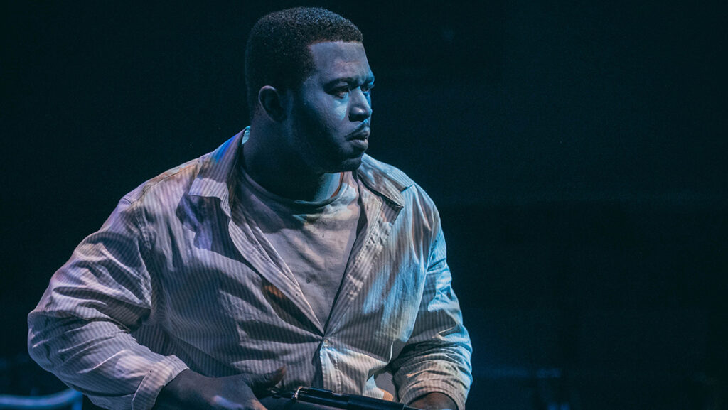
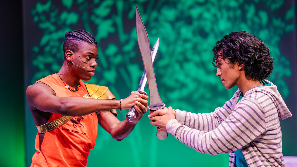
UNCG Summer Arts and Design Intensive
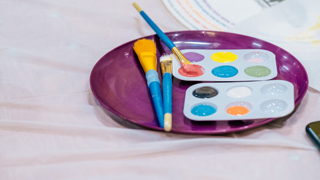
UNCG’s Summer Arts and Design Intensive camp (SADI) is a residential art program for young artists. SADI covers various art forms such as drawing, painting, printmaking, sculpture, photography, graphic design, and animation. Students in grades 8 through 12 work alongside UNCG School of Art faculty, art education staff, and the Weatherspoon Art Museum to engage in college-level studio classes and create portfolio-quality artwork. The dates for UNCG Arts and Design Intensive camp are July 14 – 19.
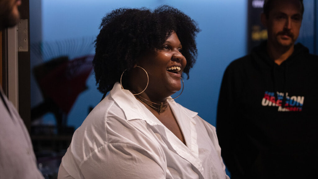
“On a personal level, working at the camp has deepened my appreciation for the resilience and strength of children despite facing numerous challenges.”
Melina Sneesby, DREAM volunteer
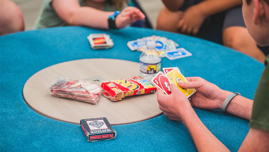
UNCG Esports and Gaming camp
UNCG Esports and Gaming camp is a summer program for ages 8-14 and 13-17. These seven one-week camps are offered on campus in the Esports Arena and computer lab spaces. In addition, a new camp, Unreal Engine Gaming Academy, kicks off this year for ages 13-17. Campers focus on two subjects each week with plenty of free time for gameplay and friendly competitions. The dates for UNCG Esports and Gaming camp are June 17 – August 2.
Technovation for Good
Technovation for Good, made possible by Alex Lee, Inc. is a day and residential program for rising high school sophomores – seniors. The program is administered by the Information Systems and Supply Chain Management department at the Bryan School of Business and Economics. Students experience hands-on learning in programming, cybersecurity, data analytics, mobile app development, sustainability, analytics, and more. Promoting inclusiveness and education equity, students can expect to hear from local professionals, meet other students, and attend workshops to enhance their information technology and business skills. The dates for Technovation for Good are June 22 – July 2.
“I have experienced and witnessed firsthand how guidance and encouragement can empower students to overcome obstacles and achieve their goals.”
Agustin Saldana, CHANCE volunteer
DREAM camp
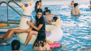
DREAM is a day camp for children and adolescents ages 8 to 18 with social and friendship challenges, including, but not limited to, those with high-functioning autism. The focus is to engage campers in a community that fosters development and enhances their life skills. Campers will take part in arts and crafts, musical performances, and sports. The dates for DREAM camp are June 17 – 21 and July 8 – 12 from 9 a.m. – 3 p.m.
Camp Speak-a-lot
Camp Speak-a-lot is a free program designed for children who stutter, ages 7-13. Located at UNCG’s Piney Lake, researchers from the UNCG Department of Communication Sciences and Disorders help to guide children through questionnaires about mindfulness and their thoughts and feelings related to stuttering, seeking to improve future therapy outcomes. Camp activities include art, theatre, hiking, games, water activities, and yoga. The dates for Camp Speak-a-lot are June 17 – 28 from 1 p.m. to 4 p.m. For more information on how to register, reach out to Kelly Harrington at ktharrin@uncg.edu.
Listening Lab
Listening Lab is a program designed for children with (central) auditory processing disorder, ages 7-12. Located at UNCG’s Speech and Hearing Center, supervising clinicians focus on strengthening foundational auditory skills needed for listening, learning, and communication. Campers rotate through listening stations and receive group and/or individual training in various areas. The dates for Listening Lab are June 17 – 28 from 1 p.m. to 4 p.m. For more information on how to register, reach out to Lisa Fox-Thomas at lfoxthomas@csdshc.uncg.edu.
“The most fulfilling thing about volunteering with DREAM camp was being able to see our campers achieve the goals that they had set at the start of the week for camp.”
Gregory Chase, DREAM volunteer
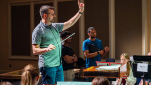
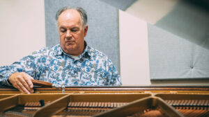
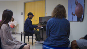
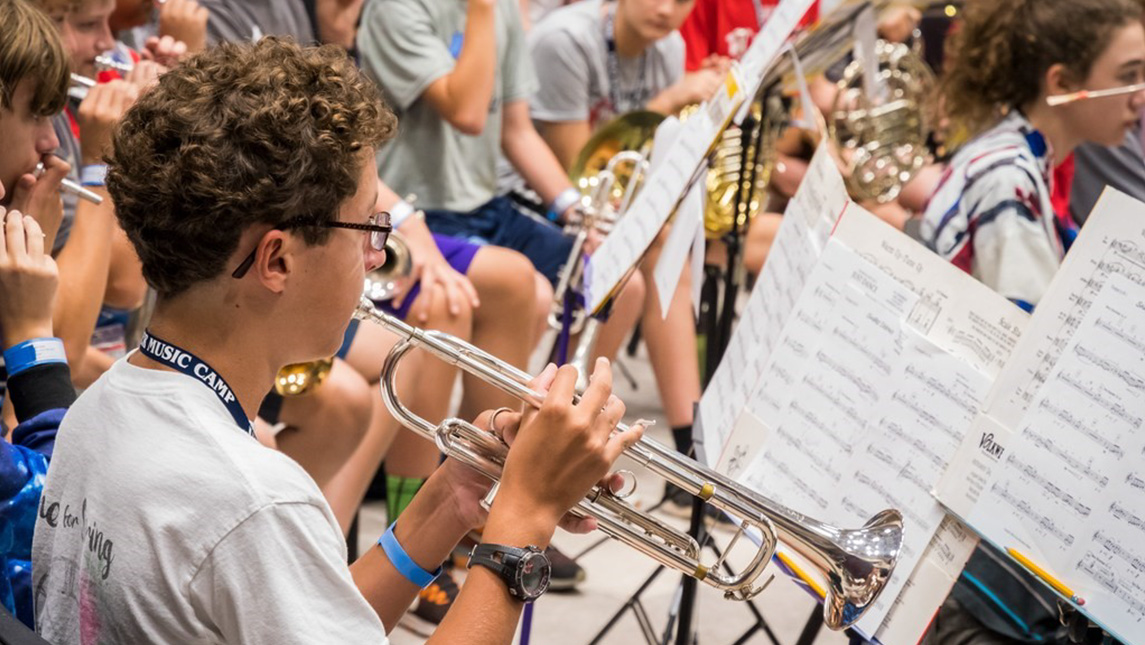
UNCG Summer Music Camp
UNCG Summer Music Camp offers a two-week program in band, mixed chorus, orchestra, and piano. Students work with artist-faculty of the UNCG School Of Music and other music teachers, performers, and conductors throughout the state and nation. Each camp concludes on Friday with a concert for parents, relatives, friends, and community members. The dates for UNCG Music Camp are July 7 – 12 and July 14 – 19.
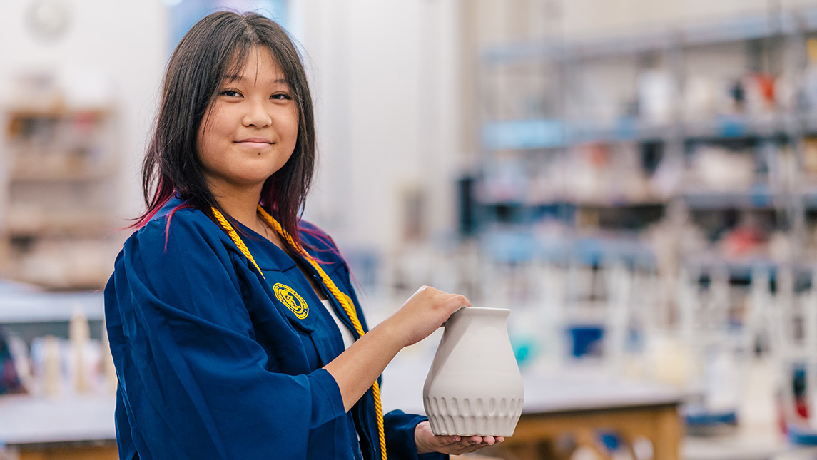
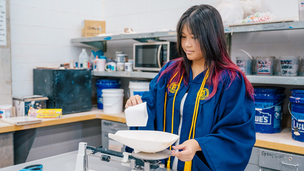
JSNN ExPlorers Summer Camp
The Joint School of Nanoscience and Nanoengineering (JSNN) is where innovation and interdisciplinary research converge to tackle pressing global challenges. JSNN ExPlorers Summer Camp is a free one-week program for high school students in grades 10-12 with a passion for STEM. With an emphasis on Phosphorus sustainability, students connect STEM concepts to real-world experiences in the classroom. Camp activities include gaining laboratory experience, developing 3D printing skills, visiting a local farm, and attending college tours. The dates for JSNN ExPlorers Summer Camp are July 8 – 12 from 9 a.m. to 4 p.m.
UNCG Sports
UNCG hosts several summer sports camps run by the UNCG coaching staff. Click the link below for more information on programs for different sports and ages, session dates, contact information, and links to register.
“In the program, we were able to accommodate many types of students with a variety of backgrounds, abilities, and preferences. It was exciting to see the interest and commitment many of the students had towards their future in college.”
Paige Terwilliger, Arts and Design Intensive volunteer
Story by Lauren Segers, University Communications
Photography by Sean Norona and David Lee Row, University Communications